I/O
Inputs
The code requires several input files, depending on the settings chosen in the yaml
configuration file.
Intrinsic Alignment.
In the eNLA model, the parameter \(\beta_{\rm IA}\) regulates the redshift scaling of the luminosity ratio \(\left[ \langle L \rangle(z) / L_{\star}(z) \right]\):
\[P_{\delta {\rm IA}}(k, z)= - \frac{ \mathcal{A}_{\rm IA} C_{\rm IA} \Omega_{\rm m,0} \mathcal{F}_{\rm IA}(z) }{ D(z) } P_{\delta \delta}(k, z)\]where the redshift evolution is given by
\[\mathcal{F}_{\rm IA}(z) = \left( \frac{1+z}{1+z_{\rm pivot}} \right)^{\eta_{\rm IA}} \left[ \langle L \rangle(z) / L_{\star}(z) \right]^{\beta_{\rm IA}}\]If \(\beta_{\rm IA}\) is different from zero, a file with the values of the luminosity ratio as a function of redshift should be provided. This file should have two columns, the first one containing the redshift and the second one the luminosity ratio. Its location can be specified in the configuration file:
intrinsic_alignment:
   bIA: 0.0
   lumin_ratio_filename: null
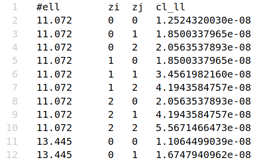
\(\boldsymbol{C_{ij}(\ell)}\)
The input \(C_{ij}(\ell)\) can be provided as an external input to compute the Gaussian covariance. In this case, the input files should be provided in the following format:
first column: \(\ell\) values
second column: index of the i-th redshift bin
third column: index of the j-th redshift bin
fourth column: \(C_{ij}(\ell)\) value
A couple words of caution in this case:
Even when input \(C_{ij}(\ell)\) are used, the code will compute radial kernels to project the non-Gaussian covariance trispectra. The user should make sure that the input cls match the cosmology and systematics defined in the configuration file. To facilitate this comparison, a plot comparing the input (auto-ij) \(C_{ij}(\ell)\) to the internally computed ones (either with
CLOEorCCL) will be produced when running the code with the--show-plotsflag.The input \(C_{ij}(\ell)\) will be interpolated with splines in the \(\ell\) values required in the cfg file; for this, the Cls should be sampled on a sufficiently large number of \(\ell\) points.
C_ell:
   use_input_cls: True
   cl_LL_filename: ./input/cl_ll.txt # shear-shear
   cl_GL_filename: ./input/cl_gl.txt # galaxy-shear
   cl_GG_filename: ./input/cl_gg.txt # galaxy-galaxy
Galaxy and magnification bias.
The values of \(b_g(z)\) and \(b_m(z) = 5s(z)-2\), with \(s(z)\) the logarithmic slope of the lenses’ luminosity function for the given selection. These files should have
zbins + 1columns, the first one containing the redshift and the remaining ones the value of the bias in each redshift bin (these values can coincide). The location of these files can be specified in the configuration file:C_ell: gal_bias_table_filename: ./input/gal_bias.txt mag_bias_table_filename: ./input/mag_bias.txt
If these files are not provided, the code will use a third-order polynomial fit of the form:
\[b_X(z) = a_{X, 0} + a_{X, 1} \, z + a_{X, 2} \, z^2 + a_{X, 3} \, z^3\]where \(X\) can be either
gorm. The coefficients \(a_{X, i}\) can be specified in the configuration file.For the galaxy bias, we also provide the option to use the galaxy bias computed from the HOD model through
CCL. In the last two cases (polynomial bias and HOD bias), the bias will be the same in all redshift bins., i.e. \(b^i_{X}(z) = b^j_{X}(z)\).Mask
The mask can be provided in
.fitsor.npyformat. Additionally, the code offert the possibility to generata a circular footprint covering the survey area and with thensidespecified in the configuration file. The footprint should normally be a binary mask; a non-binary footprint is accepted but interpreted as fractional weighting (effective fsky =mean(W_a * W_b), TJPCov convention). Note that ifnsideis not None, it will also be used to adjust the resolution of the input mask, either upgrading or downgrading it as needed.mask: use_footprint: False mask_filename: ../input/mask.fits generate_polar_cap: True nside: 1024 survey_area_deg2: 13245
Outputs
Covariance
The main output of Spaceborne is the covariance matrix for the requested probes
(lensing, photometric galaxy clustering, ggl), terms (Gaussian and its components
– SVA, SN, MIX –, plus the non-Gaussian terms SSC and cNG)
and statistics (C_ells, 2PCF). The path to the output folder can be specified in the
configuration file; the file format is .npz, for maximum storage
efficiency. These files can be loaded as arrays with
covs_2d = np.load(f'{cov_filename}_2D.npz')
With cov_filename specified in the config file:
covariance:
   cov_filename: 'my_covs'
You can then inspect the files in the archive with covs_2d.files. The different
entries will correspond to the different terms of the covariance, depending on the ones
requested in the config file. For example, if we required the Gaussian and super-sample
covariance terms, we will have
[in]  covs_2d.files
[out] ['Gauss', 'SSC', 'TOT']

[in]  cov_g_2d = covs_2d['Gauss']
[in]  cov_g_2d.ndim
[out] 2
The probes present in each of these 2D arrays will instead depend on the probes
selected in the probe_selection section.
The order along the diagonal will always follow the one in the config file
(i.e.: LLLL, then GLGL, then GGGG for harmonic space;
xip, xim, gt and w for real space).
In any case, some plots are produced at runtimes with labels to help distinguish the
different probe blocks.
To better understand the ordering of the covariance matrix elements in the 2D
representation, we note that in general, given a certain probe combination ABCD,
the covariance matrix can be described by a 6-dimensional array
with axes cov_ABCD[s1, s2, zi, zj, zk, zl]. In this representation:
The first and second axes index the angular scales \(\ell_1\) and \(\ell_2\), or \(\theta_1\), \(\theta_2\).
The last four axes index the redshift bins \(z_i, z_j, z_k, z_l\).
The redshift indices can then be compressed leveraging the symmetry of the auto-spectra:
taking the harmonic space case as an example,
\(C_{ij}^{AA}(\ell) = C_{ji}^{AA}(\ell)\). This simply means taking the
upper or lower triangle of the \(C_{ij}(\ell)\) matrix (for each \(\ell\)),
in a row-major or column-major fashion.
This is the meaning of the triu_tril and row_col_major
options in the configuration file. Compressing the covariance matrix in this way will
result in an four-dimensional array with axes
cov_ABCD[s1, s2, zij, zkl], with zij and zkl indexing the unique
redshift pairs. To create a 2D array, we can simply flatten by looping over the
different indices; to do this, we need to choose the order of the loops, which will
determine the structure of the 2D covariance matrix. This can be specified with the
covariance_ordering_2D key in the configuration file. The possible options are:
scale_probe_zpair: the angular scale index (\(\ell\) or \(\theta\)) will be the outermost one, followed by the probe and the redshift pair indices.probe_scale_zpair: the probe index will be the outermost one, followed by the scale and the redshift pair indices.
Even knowing the structure of the 2D covariance in detail, retrieving specific
elements can be a bit cumbersome (say we want to have a look at the
zi, zj, zk, zl = 0, 1, 0, 1 slice of the LLLL block). To
make life easier for the user, the code offers the possibility to save the covariance
matrix as an npz archive of 6D arrays. This can be done by setting
covariance:
   save_full_cov: true
in the config file. The archive will now consist of one 6D array for each unique probe combination and for each term of the covariance matrix:
[in] covs_6d = np.load(f'{cov_filename}_6D.npz')
[in] covs_6d.files
[out] ['LLLL_Gauss', 'LLLL_SSC', 'LLLL_TOT',
       'LLGL_Gauss', 'LLGL_SSC', 'LLGL_TOT',
       'LLGG_Gauss', 'LLGG_SSC', 'LLGG_TOT',
       'GLGL_Gauss', 'GLGL_SSC', 'GLGL_TOT',
       'GLGG_Gauss', 'GLGG_SSC', 'GLGG_TOT',
       'GGGG_Gauss', 'GGGG_SSC', 'GGGG_TOT']

[in]  cov_llll_g_6d = covs_6d['LLLL_Gauss']
[in]  cov_llll_g_6d.ndim
[out] 6
Please note that this format will produce larger files.
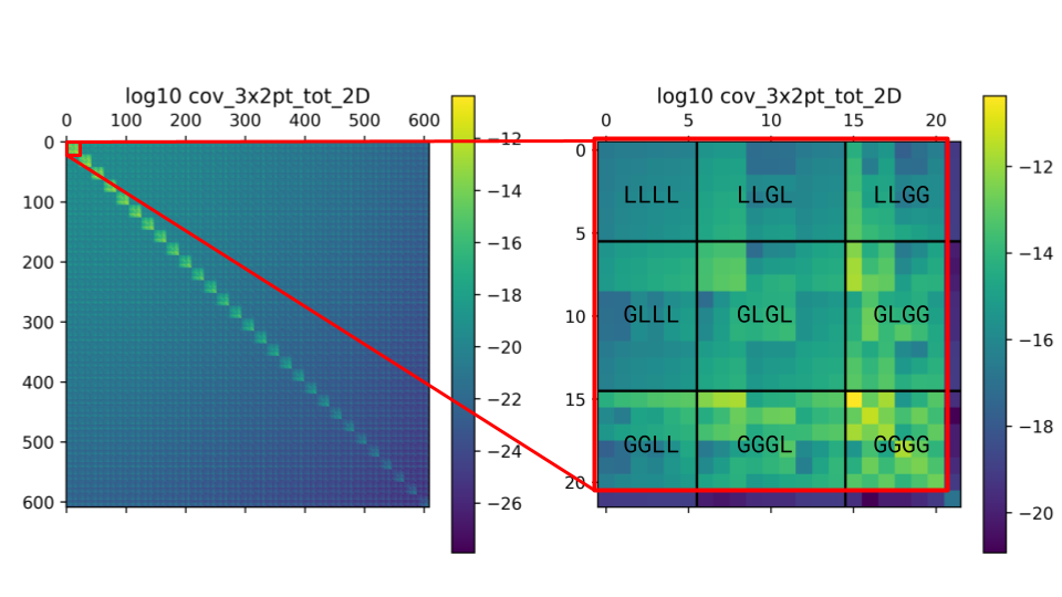
Example of the 2D covariance matrix for the scale_probe_zpair ordering scheme.
These plots display the log10 of the absolute value of the covariance matrix elements.
In this ordering, the blocks visible in the left panel correspond to the
different \(\ell_1-\ell_2\) combinations (“ell-blocks”);
the off-diagonal blocks are due to the presence of SSC, in this example.
Zooming into the first diagonal block (right
plot), we can discern the sub-blocks corresponding to the different probe combinations
(specified in the figure). Finally, within each “probe-block”, the individual
elements correspond to the different redshift pairs.
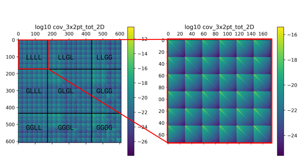
Example of the 2D covariance matrix for the probe_zpair_scale (in the label,
probe_zpair_ell) ordering scheme.
These plots display the log10 of the absolute value of the covariance matrix elements.
In this ordering, the blocks highlighted in the left panel correspond to the
different probe combinations (“probe-blocks”, labeled in the figure).
Zooming into the first diagonal block (right
plot), we can discern the sub-blocks corresponding to the different redshift pair
combinations (there are N=3 redshift bins in this case, which for the auto-spectra
correspond to \(N(N+1)/2=6\) unique pairs). Finally, within each “zpair-block”,
the individual elements correspond to the different \(\ell_1-\ell_2\) combinations.
Again, the off-diagonal elements within the “ell-blocks” are due to the presence of SSC.
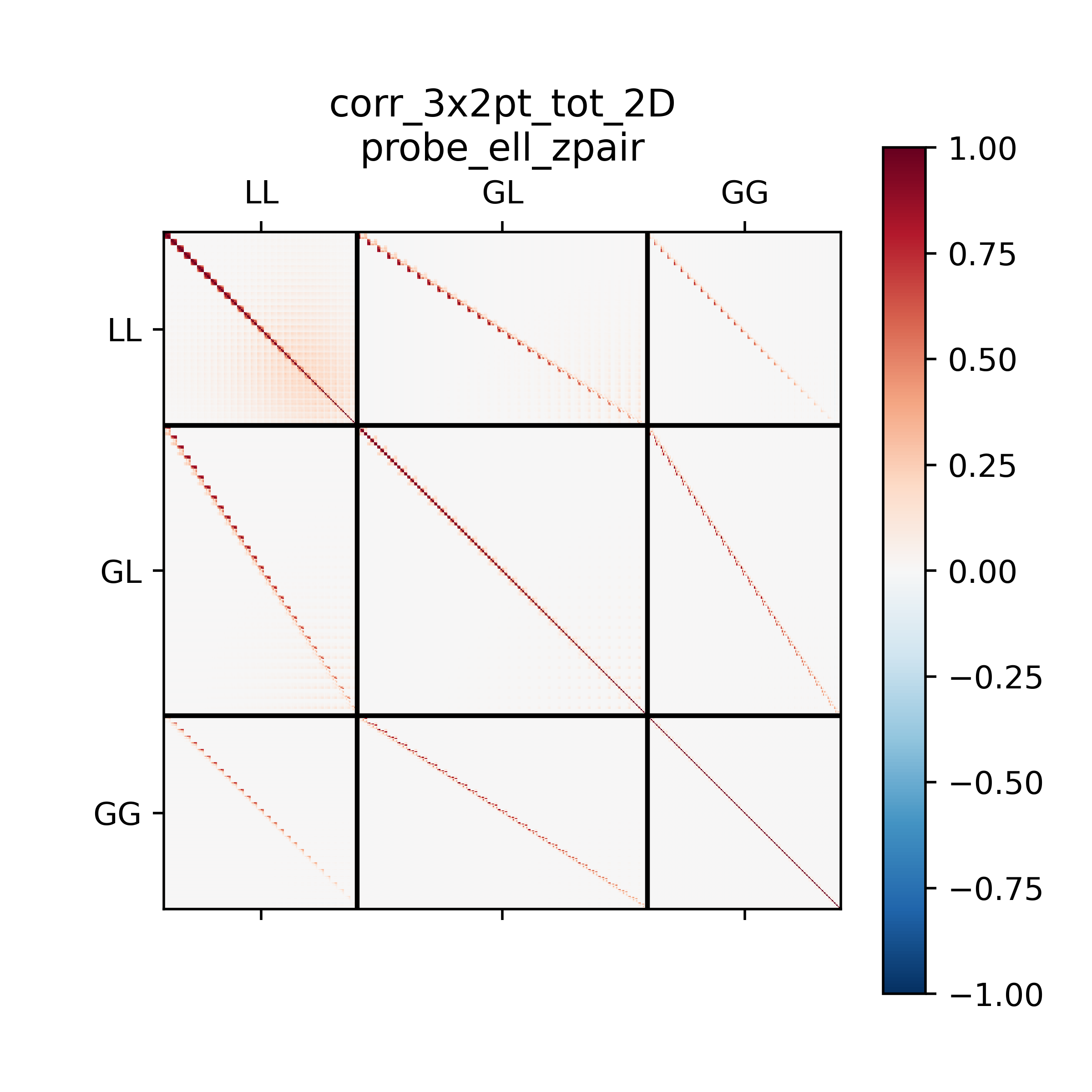

Further examples of the 2D orderings, this time displaying the correlation matrix.
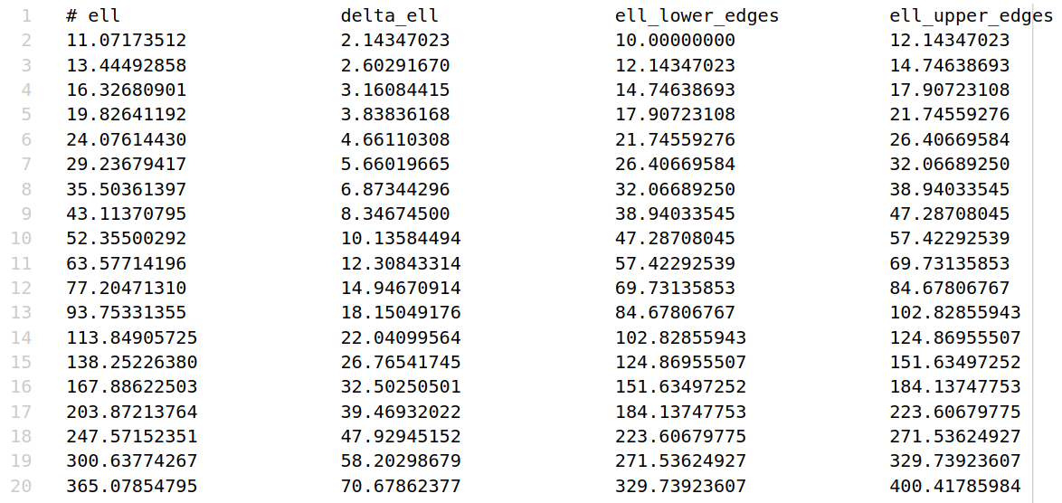
\(\ell\) values
Another output of the code is the multipoles at which the covariance matrix is computed,
along with the full specifics of the \(\ell\) binning scheme adopted (bin width
and edges). These can be found in the ell_values_<probe>.txt files.
\(C_{ij}(\ell)\)
The \(C_{ij}(\ell)\) are also saved as plain .txt files, with the same format as
for the input (see point 2 of “Inputs” section).
run_config.yaml
The last output of the code is the run_config.yaml file, which contains the configurations
used to run the code. This can be useful to reproduce the same run in the future,
as well as to have a reference of the exact settings used.